Fire from above

Using Google Earth Engine's python API, I analyse fires over the last twenty years in a protected area in Malawi.

Here, we used the Earth Engine version of the Fire Information for Resource Management System (FIRMS) dataset, showing near real-time (NRT) active fire locations which each representing the centroid of a 1 km pixel that is flagged by the algorithm as containing one or more fires within the pixel.

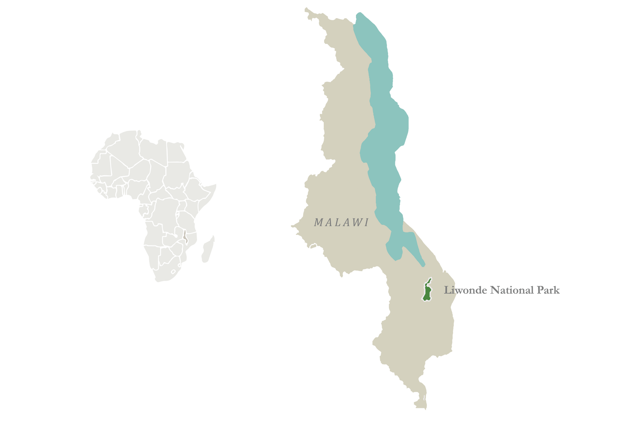
Focusing on Liwonde, Malawi

Liwonde National Park at 548 km² is part of the Great East African Rift Valley in southern Malawi. With Mopane dominated woodland, some floodplains, grasslands and riverine forests and thickets, Liwonde provides a diverse habitat for many species.

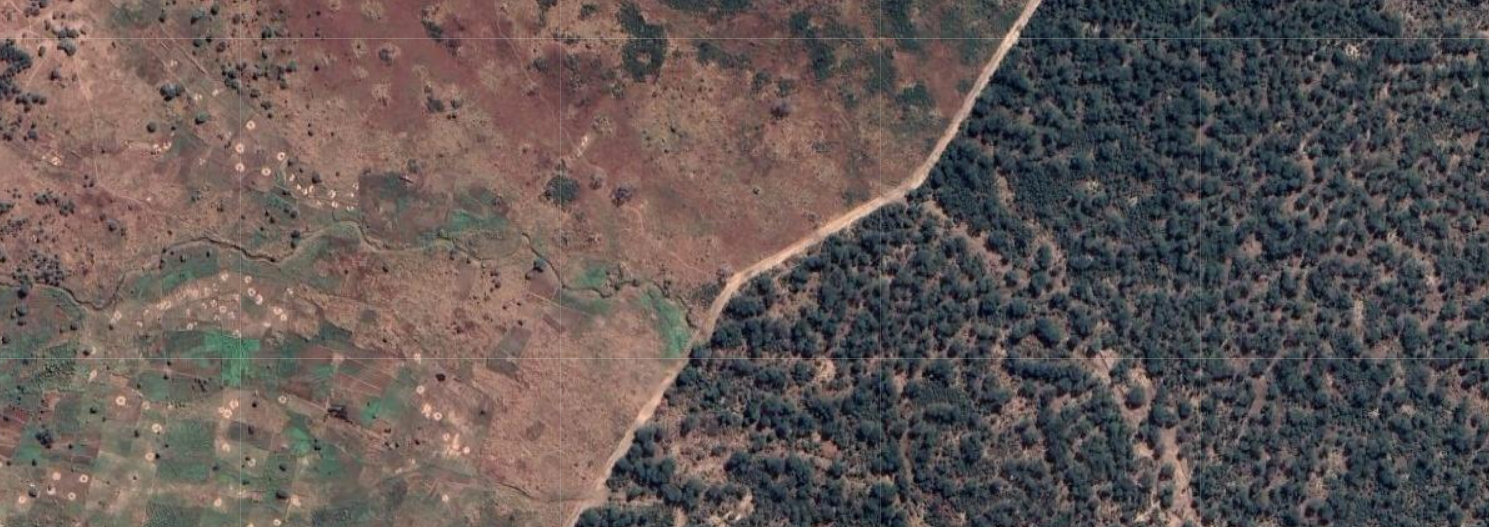
However, in Malawi, there are typically very hard boundaries between protected areas and surrounding communities. A fence often separates lush woodlands and people living in poverty. Fires made by people often spread into the protected area leading to frequent burning of vegetation which can shift habitats to different states, i.e. from woodlands to grasslands.

Getting started with the fire analysis

Let's import the relevant packages and specify the projection to get going.

# Installs geemap package
import ee
import subprocess
import geemap
import fiona
import seaborn as sbn
import matplotlib.pyplot as plt

# We use WGS 84 / Pseudo-Mercator
project_crs = 'EPSG:3857'
project_projection = ee.Projection(project_crs)

Create a water mask

Using the JRC Yearly Water Classification History, we create a water mask to use later.

water = ee.ImageCollection('JRC/GSW1_3/YearlyHistory').filterDate('2010-01-01', '2021-01-01').median()
water_mask = water.gt(1.0).selfMask().unmask()
water_mask = water_mask.eq(0).selfMask()

Import shapefile of the area of interest

An easy way to import a file into the Colab Notebook is by adding it to Google Drive. The below code will trigger a popup for you to connect to Google Drive.

from google.colab import drive
drive.mount('/content/drive')

Then, you can upload the geojson file to Google Drive and easily import into the Notebook.

park_name = 'Liwonde National Park'

parks = []
with open("/content/drive/MyDrive/data/Boundaries.geojson") as f:
    json_data = json.load(f)
    for feature in json_data['features']:
      # print(feature['properties']['name'])

      if feature['properties']['name'] == park_name:
        feature['properties']['style'] = {}
        parks.append(feature)

park = geemap.geojson_to_ee(parks[0])
print(park)

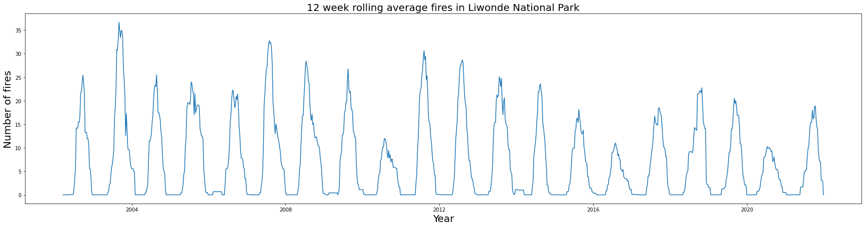
Fire timeseries

For the Liwonde area of interest, we aggregated all fire pixels in 7-day time periods. Using a 12 week rolling average, we obtain a smooth overlay as below.

from datetime import datetime
import pandas as pd 
import ee

img_date_range = [d.strftime('%Y-%m-%d') for d in pd.date_range('2002-01-01', '2022-01-01', freq='7d')]

img_date_list = ee.List(img_date_range)

def create_img_for_week(day):
  fire_image = ee.ImageCollection('FIRMS').filter(ee.Filter.date(ee.Date(day), ee.Date(day).advance(7, 'day'))).select('T21')
  fire_info = fire_image.first()
  fire = fire_image.count().gt(0);
  fire = fire.copyProperties(fire_info, ['system:time_start', 'system:footprint', 'system:time_end', 'system:version', 'system:id', 'system:asset_size', 'system:index', 'system:bands', 'system:band_names'])
  return fire

weekly_images = ee.ImageCollection(img_date_list.map(create_img_for_week))

def poi_mean(img):
    count = img.reduceRegion(reducer=ee.Reducer.count(), geometry=park, scale=1000).get('T21')
    return img.set('date', img.date().format()).set('count', count)

weekly_fires = weekly_images.map(poi_mean)



nested_list = weekly_fires.reduceColumns(ee.Reducer.toList(2), ['date','count']).values().get(0)

window = 12

df = pd.DataFrame(nested_list.getInfo(), columns=['date','count'])
df['date'] = pd.to_datetime(df['date'])
df['rolling'] = df.rolling(window).mean()

fig, ax = plt.subplots(figsize=(30,7))
sbn.lineplot(data=df, ax=ax, x='date', y='rolling')
# sbn.set(font_scale=2, font="Verdana")

ax.set_ylabel('Number of fires',fontsize=20)
ax.set_xlabel('Year',fontsize=20)
ax.set_title('12 week rolling average fires in '+ park_name ,fontsize=20);
from matplotlib.colors import LinearSegmentedColormap

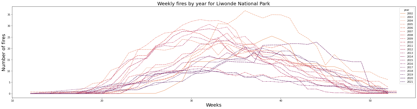
Weekly fires by year

Here, we try to get an idea if the burning season has shifted earlier or later in comparison to previous years.

from matplotlib.colors import LinearSegmentedColormap

year_df = df
year_df['year'] = pd.DatetimeIndex(year_df['date']).year
year_df['month'] = pd.DatetimeIndex(year_df['date']).month
year_df['week'] = pd.DatetimeIndex(year_df['date']).week
year_df = year_df[['date', 'week', 'count', 'year']]

pivot_df = year_df.pivot_table(index='week', columns='year', values='count', aggfunc='sum')

cpal = sbn.color_palette("flare", 20)

fig, ax = plt.subplots(figsize=(30,7))
g = sbn.lineplot(data=pivot_df.rolling(12).mean(), ax=ax, palette=cpal)
ax.set_ylabel('Number of fires',fontsize=20)
ax.set_xlabel('Weeks',fontsize=20)
ax.set_title('Weekly fires by year for '+ park_name ,fontsize=20);

From 2002 to about 2014, burning started as early as Week 20 (17 May), with peak burning season starting in Week 24 (14 June) until Week 38 (20 September), with the last fires in Week 50 (13 December). From 2014 to about 2021, burning generally started later and fewer fires are recorded. Burning started as early as Week 23 (7 June), with peak burning season only starting in Week 32 (9 August) until Week 45 (8 November), with the last fires in Week 50 (13 December). One can assume that the later in the season the fire occurs, the more intense it is.

Comparing the burning season with rainfall

One would expect that burning happens during the drier season. Let's see what we find.

rainfall = ee.ImageCollection('WORLDCLIM/V1/MONTHLY')

def poi_mean(img):
    mean = img.select('prec').reduceRegion(reducer=ee.Reducer.mean(), geometry=park, scale=1000).get('prec')
    return img.set('prec', mean).set('date', img.metadata('month'))

monthly_rainfall = rainfall.map(poi_mean)

nested_list = monthly_rainfall.reduceColumns(ee.Reducer.toList(2), ['prec','month']).values().get(0)

df = pd.DataFrame(nested_list.getInfo(), columns=['prec','month'])
    
new_df = df[['prec', 'month']]
fig, ax = plt.subplots(figsize=(30,7))
g = sbn.lineplot(data=new_df, x='month', y='prec', ax=ax)
# g.set_xticklabels(['6','8','10','12','2','4','6'])
ax.set_ylabel('Rainfall (mm)',fontsize=20)
ax.set_xlabel('Month of the year',fontsize=20)
ax.set_title('Average monthly rainfall',fontsize=20);

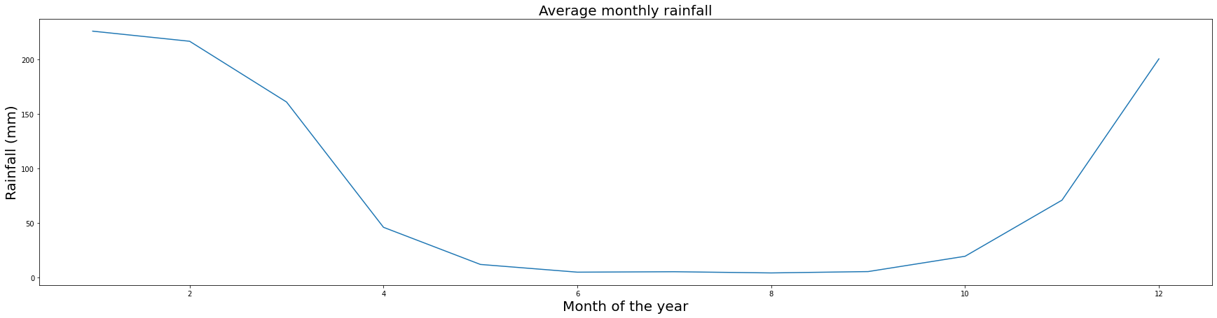
This confirms that burning starts when rainfall levels begin to drop.

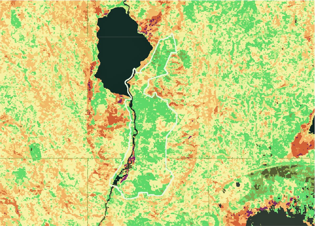
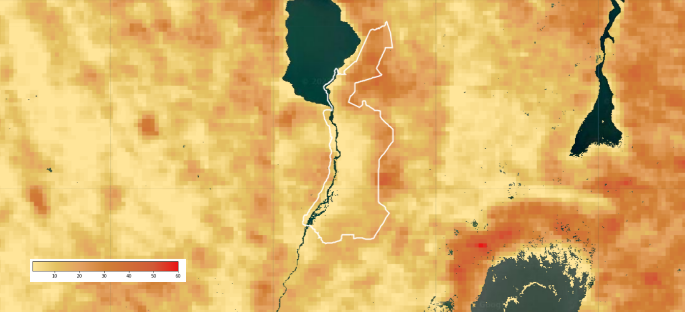
Burn frequency

Here, we count how many times in a year a pixel burnt and also use the water mask we created earlier. We created 14-day periods and checked if a pixel burned during that time. Then we checked for how many of the 14-day periods a pixel burned during the year. Thus, the maximum number is 26 times a pixel could've burned during the year. This analysis was conducted from 2002-01-01 until 2022-01-01, meaning the ultimate maximum value of a pixel is 520 as there are 520 two-week periods in 20 years.

from datetime import datetime
import pandas as pd 
import ee

img_date_range = [d.strftime('%Y-%m-%d') for d in pd.date_range('2002-01-01', '2022-01-01', freq='14d')]
img_date_list = ee.List(img_date_range)


def create_img_for_day(day):
  fire_image = ee.ImageCollection('FIRMS').filter(ee.Filter.date(ee.Date(day), ee.Date(day).advance(14, 'day'))).select('T21').sum().gt(0);
  return fire_image

doy_images = ee.ImageCollection(img_date_list.map(create_img_for_day))

project_proj = doy_images.mean().projection()

fire = doy_images.sum().reproject(project_projection, None, 1000).reduceResolution(
      reducer = ee.Reducer.sum(),
      )
firewatermask = fire.mask(water_mask)

We can then map the output into an interactive map:

Map = geemap.Map()
Map.addLayer(firewatermask, {'min':1, 'max':60, 'palette':['#ffe599', '#e4c261', '#e4a161', '#d18236', '#d16d36', '#d15936', '#ea1616']}, 'fires')
park_fc = ee.FeatureCollection(park)
Map.addLayer(park_fc.style(color='white', fillColor='00000000'))
Map.setCenter(35.337005, -14.924659, 9)
Map

The resulting map shows that the Northern and Eastern boundaries of the park burn most frequently. Interestingly, the surroundings outside the protected area does not burn significantly more frequent. This may be because there is just less fuel such as dense vegetation for fires to consume.

Burn scar mapping

Here we obtain Sentinel-2 data for the year of 2021 and mask all clouds and cloud shadows. Below are a few helpful cloud and shadow masking functions we'll use.

def get_s2_sr_cld_col(datefilter):
    s2_sr_col = (ee.ImageCollection('COPERNICUS/S2_SR')
        .filter(datefilter)
        .filter(ee.Filter.lte('CLOUDY_PIXEL_PERCENTAGE', CLOUD_FILTER)))

    s2_cloudless_col = (ee.ImageCollection('COPERNICUS/S2_CLOUD_PROBABILITY')
        .filter(datefilter))

    return ee.ImageCollection(ee.Join.saveFirst('s2cloudless').apply(**{
        'primary': s2_sr_col,
        'secondary': s2_cloudless_col,
        'condition': ee.Filter.equals(**{
            'leftField': 'system:index',
            'rightField': 'system:index'
        })
    }))


def add_cloud_bands(img):
    cld_prb = ee.Image(img.get('s2cloudless')).select('probability')
    is_cloud = cld_prb.gt(CLD_PRB_THRESH).rename('clouds')
    return img.addBands(ee.Image([cld_prb, is_cloud]))


def add_shadow_bands(img):
    # Identify water pixels from the SCL band.
    not_water = img.select('SCL').neq(6)

    # Identify dark NIR pixels that are not water (potential cloud shadow pixels).
    SR_BAND_SCALE = 1e4
    dark_pixels = img.select('B8').lt(NIR_DRK_THRESH*SR_BAND_SCALE).multiply(not_water).rename('dark_pixels')

    # Determine the direction to project cloud shadow from clouds (assumes UTM projection).
    shadow_azimuth = ee.Number(90).subtract(ee.Number(img.get('MEAN_SOLAR_AZIMUTH_ANGLE')));

    # Project shadows from clouds for the distance specified by the CLD_PRJ_DIST input.
    cld_proj = (img.select('clouds').directionalDistanceTransform(shadow_azimuth, CLD_PRJ_DIST*10)
        .reproject(**{'crs': img.select(0).projection(), 'scale': 100})
        .select('distance')
        .mask()
        .rename('cloud_transform'))

    # Identify the intersection of dark pixels with cloud shadow projection.
    shadows = cld_proj.multiply(dark_pixels).rename('shadows')

    # Add dark pixels, cloud projection, and identified shadows as image bands.
    return img.addBands(ee.Image([dark_pixels, cld_proj, shadows]))

def add_cld_shdw_mask(img):
    # Add cloud component bands.
    img_cloud = add_cloud_bands(img)

    # Add cloud shadow component bands.
    img_cloud_shadow = add_shadow_bands(img_cloud)

    # Combine cloud and shadow mask, set cloud and shadow as value 1, else 0.
    is_cld_shdw = img_cloud_shadow.select('clouds').add(img_cloud_shadow.select('shadows')).gt(0)

    # Remove small cloud-shadow patches and dilate remaining pixels by BUFFER input.
    # 20 m scale is for speed, and assumes clouds don't require 10 m precision.
    is_cld_shdw = (is_cld_shdw.focalMin(2).focalMax(BUFFER*2/20)
        .reproject(**{'crs': img.select([0]).projection(), 'scale': 20})
        .rename('cloudmask'))

    # Add the final cloud-shadow mask to the image.
    return img_cloud_shadow.addBands(is_cld_shdw)


def apply_cld_shdw_mask(img):
    # Subset the cloudmask band and invert it so clouds/shadow are 0, else 1.
    not_cld_shdw = img.select('cloudmask').Not()

    # Subset reflectance bands and update their masks, return the result.
    return img.select('B.*').updateMask(not_cld_shdw)

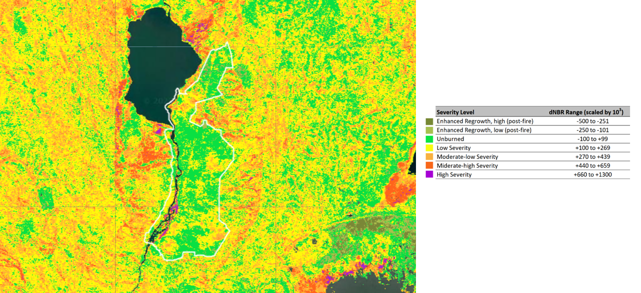
We choose the peak of the fire season as 2021-10-03, specifying the overall burning season from 2021-06-15 to 2021-12-10. For the month before the burning season (pre-burn) we calculated the Normalised Burn Ratio (NBR), as well as for the month after the burning season (post-burn)

CLOUD_FILTER = 40
CLD_PRB_THRESH = 50
NIR_DRK_THRESH = 0.15
CLD_PRJ_DIST = 1
BUFFER = 50

burn_date = '2021-10-03'
before_date_filter = ee.Filter.date(ee.Date(burn_date).advance(-4, 'months'), ee.Date(burn_date).advance(-2, 'months'))
after_date_filter = ee.Filter.date(ee.Date(burn_date).advance(2, 'months'), ee.Date(burn_date).advance(4, 'months'))

sentinel_before_burn = get_s2_sr_cld_col(before_date_filter).filterBounds(park).map(add_cld_shdw_mask).map(apply_cld_shdw_mask).mean()
sentinel_after_burn = get_s2_sr_cld_col(after_date_filter).filterBounds(park).map(add_cld_shdw_mask).map(apply_cld_shdw_mask).mean()


before_nbr = sentinel_before_burn.normalizedDifference(['B8', 'B12'])
after_nbr = sentinel_after_burn.normalizedDifference(['B8', 'B12'])

dNBR = before_nbr.subtract(after_nbr).multiply(1000)
dNBR = dNBR.mask(water_mask)

thresholds = ee.Image([-1000, -251, -101, 99, 269, 439, 659, 2000]);
scar_classes = dNBR.gt(thresholds).reduce('sum').toInt();

Let's map the result.

Map = geemap.Map()
Map.addLayer(dNBR, {'palette':['white', 'black']}, 'nbr')
Map.addLayer(scar_classes, {'min':0, 'max':7, 'palette':['#ffffff','#7a8737', '#acbe4d', '#0ae042', '#fff70b', '#ffaf38', '#ff641b', '#a41fd6']}, 'scars')
park_fc = ee.FeatureCollection(park)
Map.addLayer(park_fc.style(color='white', fillColor='00000000'))
Map.setCenter(35.337005, -14.924659, 9)
Map

What's next?

I would like to build an interactive fire mapping app providing a self-service to users, something like this prototype with Google Earth Engine.